INTRODUCTIONSince the discovery of evoked otoacoustic emissions (OAE) by Kemp in 1978, the method has now been implemented as a daily routine test in most clinics and has been incorporated as a valuable tool in the audiological test-battery. One of the most important applications for the transient evoked otoacoustic emissions method (TEOAE) is the ability to detect hearing losses in neonates. A practical problem, however, in testing babies or young children using TEOAEs, is the demand for the child to be quiet for one or two minutes during the examination. In the conventional TEOAE procedure the recording window is normally 20 ms allowing for a maximum stimulus rate of 50 stimuli per second. Furthermore, in order to achieve a realistic signal-to-poise ratio 2-3000 responses are required to be averaged. In a clinicai situation one replication of the investigation is normally carried out, which means that at least 2 minutes of test time is necessary. In practise, however, restless and noisy babies can easily take 10 minutes or more to test due to rejection of responses contaminated with acoustical noise and movement artifacts.
In 1982 Eysholdt and Schreiner suggested the use of maximum length sequences (MLS) for recording auditory brain stem responses. By this technique it is possible to reduce recording time by increasing the stimulus rate and to improve the signal-to-poise ratio. To overcome the difficult clinicai test situation in neonates, Thornton (1993) utilised the MLS technique to perform TEOAE measurements. Using the MLS stimulus paradigm it is feasible within a few seconds to achieve valuable sereening results in most newborns.
The purpose of this report is to describe a new designed instrument, which implements the MLS technique for recording of TEOAEs. Furthermore, different aspects of the MLS method and a new semi-non-linear recording technique will be described and discussed.
METHODSMaximum length sequences
A MLS sequence is normally generated by a shift register and an XOR gate as ilustrated in Figure 1. The shift register is initialised with +l s and hereafter the content of the register is shifted one place to the right during every time step. The left most place in the shift register (A) equals the result from the XOR operation between the two feedback connections. (A comprehensive description of MLS generation is given by Davies (1966) and Thornton (1994)).
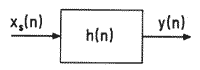
Figure 1. Shift register (ABC) for the generation of a maximum length sequence (MLS) with feedback from stage B and C via an exclusive-OR gate (XOR) to the input of the shift register (stage A).
If the feedback connections are chosen correctly, the shift register will go through ali possible states except the situation where ali stages in the register are zeros, which is a non-valid condition. A MLS sequence is only correct, if all the different possibilities are exposed that is if the sequence have a lenght equal to L=2 n - 1 where n is the number of stages in the shift register. If the time sequence from output C in a 3rd order register is chosen, then the MLS sequence will be:
Xs(n) = {1,1,1,0,0,1,0} (1)
Now, by exchange the zeros in the MLs sequence by- 1s, the so-called recovery sequence is achieved:
Xs(n) = {1,1,1, -1, -1,1, -1} (2)
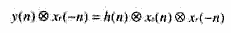
A special aspect of the MLS- and the corresponding recovery sequences is that if one of the sequences is circular convoluted with the other sequence inverted in time then the outcome will be an impulse (d(n)):
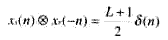
(3)
The before, if one wants to measure the impulse response of a system, it can be ìmplemented using a stimulus signal consisting of a periodic MLS sequence. For a 3rd order sequence the stimulus signal becomes:
Xstim={...1,,1,1,0,0,1,0,1,1,1,0,0,1,0,1,1,1,0,0,1,0,1,1,1,0,0,1,0...(4)
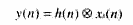
lf the duration of the impulse response is shorter than the duration of the MLS sequence, then the output signal from a system with a transfer function h(n), as shown- in Figure 2, can be written:
(5)
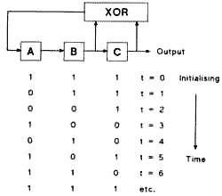
Figure 2. System with transfer function h(n) and corresponding ínput (xs(n)) and output functions (y(n)).
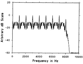
Figure 3. Frequency spectrum of the eletrical stimulus signal from as oversampled MLS-signal. The Y-axis scalling is adjusteed arbitrarily to 0 dB at the harmonic peaks os the spectrum.
lf equation (5) is convoluted on both sides with the time inverted function of the recovery signal the following expression is achieved:
(6)
By using equation (3) the expression in (6) can be written:
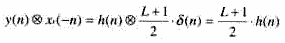
(7)
The impulse response can now be extracted by a cross correlation between the recovery signal and the output signal:
(8)
Because the recovery sequence only contains +ls and -1s the correlation can be achieved by simple additions and subtractions. In the following this correlation procedure will be denoted as a deconvolution.
Frequency resolution and stimulus rate
Application of the MLS sequence directly implies a stimulus rate of half the sampling rate, thus using a sampling rate of 16kHz, would imply a stimulus rate of 8kHz which is not applicable in a clinical situation. A solution to the problem is to modify the stimulus signal either by extending the delta functions an appropriate number of samples or by expanding the sequence by filling in zeroes. The former method can be considered as an oversampling of the sequence and subsequently convolve it by a square pulse, which implies that the spectrum is multiplied with the spectrum of the square pulse. The spectrum of a square pulse is a sin(x)/x function which is far from the desired flat stimulus spectrum.
The latter method was chosen because it only changes the stimulus spectrum slightly by superimposing harmonics of the stimulus rate. By filling in an adequate number of zeroes, the stimulus rate can be controlled while maintaining the same sampling rate.
The spectrum of the stimulus signal measured electrically is shown in Figure 3, indicating a broadband stimulus signal. The peaks in the spectrum are harmonics related to the stimulus rate.
Signal/Noise ratio
In order to get an acceptable signal to noise ratio it is necessary to use averaging, i.e. repeating the MLS sequences. The averaging may be accomplished either by summing the raw sequence of responses and then deconvolve the result afterwards or by deconvolution of each MLS sequence and then average the deconvouuted results. The latter method was selected because only this method reveals means for an efficient noise rejection process, and makes display of responses possible during the data acquisition. The disadvantage is the requirement of fast signal processing, which implies the use of a fast Digital Signal Processor.
The choice of the length of the MLS sequence is a trade-off. Longer sequences provide better performance with respect to artifacts resulting from non-linearities in the transducer system. However, the long sequences will result in loas of more data due to the abandoning of longer time intervals by the noise rejection. A sequence of 125 ms was selected as a proper compromise.
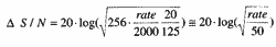
The improvement of signal to noise ratio (S/N) compared to conventional TEOAE measurements with a 20 ms time window and 50 Hz stimulus rate, using the same acquisition time, may be calculated from the following expression based on 256 stimulations pr. sequence at a click rate of 2000/s:
At a click rate of 2000/sec the S/N improvement is thus 16 dB. lf the improved S/N instead is used for acquisition time reduction, this corresponda to a reduction in time of 1/ 40 relative to the conventional TEOAE technique. Due to the reduction in the emission amplitude with increased stimulus rate, as discussed- later, the actual S/N improvement is reduced approximately 2-5 times, which means that an equivalent reduction in recording time of 8 to 20 tines relative to the conventional technique is achieved.
In neonatal screening using otoacoustic emissions, it is extremely important, for obvious reasons, to employ an efficient algorithm for the noise rejection. During data collection each new (deconvoluted) response is compared to the average result, using a calculation of the variante as the sorting parameter. The variante is calculated as the summed square of differences between the samples of the new response and the corresponding samples of the average response. A proper fixed threshold variante ïs selected for use during the data collection, but all sweeps - cancelled or accepted - are stored in memory for further analysis after the data acquisition is terminated. The problem is, that during the data collection it is impossible to select the optimal threshold variante, since by choosing a very low variante, too many responses will become discarded preventing the averaging process to provide a proper S/N. On the other hand, accepting a too high variante in the recordings will blur the average result, also resulting in a poor S/N. The point here is to find the threshold variante, which yields the best S/N. An implemented algorithm testing out a number of variante thresholds, calculates the optimal threshold variance within a few hundred milliseconds and presents the response with the optimised S/N as the final result. The rate 50 )
average effect of this optimísation during clinical conditions was observed to be within a 2-5 dB improvement of the S/ N.
Non-linear mode
Most of the conventional equivment for otoacoustic emission measurements are capable of running in the socalled "non-linear mude" in order to exclude or minimise stimulus artifacts. In the non-linear mode a measurement is first performed with 3 stimuli of the same low intensity and then hereafter an evaluation is taken with a three times higher intensity stimulus but with inverted polarity. Summing these four measurements will provide a cancellation of the stimulus. The emissions, however, do not grow in a linear fashion as a function of the stimulus intensity and will therefore not be outbalanced completely. The emissions achieved in the non-linear mode are normally smaller in amplitude than those obtained if the linear mole is used. A corresponding method was tried implemented with the MLS technique but due to auditory adaptation caused by the high stimulus rate (Thornton 1993), the generally reduced amplitudes of non-linear recordings (Bray 1989) and the constant maximum sensitivity of the system (see under Resulta), the non-linear mede was abandoned and a new hybrid solution "semi-non-linear mode" was developed,
Senu-non-linear mode
In the semi-non-linear mede the measurement is first performed for a short period of time using a 10 dB elevated stimulus intensity. This measuring step is used as a referente. Hereafter the normal recording procedure is carried out using the pre-set stimulus -intensity and the response obtained from the referente test is scaled down by the level difference between the two stimulus intensities. Then, a calculation of the power weighted cross correlation between the down scaled referente response and the emission recorded using the pre-set intensity is carried out in time intervala of 3 ms, sliding in steps of 1 ms from 0 to 10 ms in the recording window. The steps of 1 ms is chosen in order to distinguish between stimulus and emission signals with an adequate resolution. The 3 ms window is applied, to obtain a good estimate of the correlation coefficient for the actual time interval. In order to make sure that the correlation coefficient always is less than ene, a normalisation is performed with the most powerful of the two signals. In equation (9) the expression for calculatiog the povrer weighted correlation is shown:
(9)
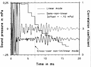
Figure 4. Comparison between two MLS recordings in an adult subject measured in linear and semi-non-linear modes. The solici curve represents the non-linear response in the time range 0-7 msec, and linear response in the remaining 13 msec of the time window. See text for further details.
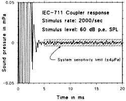
Figure 5. IEC-711 coupler response from a MLS recording. The hatched area represents the sensitivity limit of the system.
Where x represents the response using the pre-set stimulus level, y represents the downscaled reference signal resulting from the elevated stimulus level and the values with the tilde are the respective mean valises.
Because the mean value of the signals is zero, equation (9) can be simplified to:

(10)
If the recorded emissions are contaminated with a stimulus artifacts, the correlation coefficient will be high and likewise due to, that the amplitude of the emissions does not grow in a linear fashion with the stimulus level, the result will show a low correlation. From our clinicai experiences it seems like that a correlation coefficient of 0.6 is a proper divídíng line between a true response and a stimulus artifact. In the time zones where the correlation exceeds 0.6, the stimulus artifact is cancelled by subtracting the down scaled reference measurement as explained previously, and in the remaining part of the time window, the linear emission signal is left untouched.
An example demonstrating the effect of the seminon-linear mode is shown in Figure 4. The crossover point between non-linear and linear response is in this case found to be at 7 ms after stimulus onset. The semi-non linear response is shown with an offset of -0.1 mPa for clarity.
Instrumentation
The system is based on an IBM-type PC (Pentium 166 MHz) with a data acquisition module installed (National Instruments AT DSP 2200). The acquisition module comprises analogue to digital (ADC) and digital to analogue (DAC) convertera of the sigma-delta type, with 16 bit resolution and an AT&T (WE DSP32C) floating point Digital Signal Processor (DSP) with a processing power of 12.5 MIPS.
The DAC is used for stimulus signal generation and the signal is attenúated by 10 dB and buffered, before it is passed to the receiver installed in an acoustic probe (Madsen Electronics type CE-503). The microphone signal from the acoustic probe is amplified by a remote preamplifier (40 dB gain) and routed to a conditioning variable amplifier placed on a separate custorn made plug-in module in the PC. The gain is controlled via an 1/0-port in the PC in 0.375 dB steps. The microphone signal is highpass filtered with a cut-off frequency of 700 Hz and a 6 dB/octave roll-off. A second highpass filtering with cut-off frequency of 700 Hz, is accomplished using a 2.order digital IIR-filter which is optimised for a short impulse response.
The DSP and computer programs are custom made, with special emphasis on the ability of obtaining responses under severe acoustic conditions. The PC program is written in Microsoft Visual-C for Windows. The emission responses may be displayed on the screen in either time- or frequency domain and may also be printed as a report. A database is utilised (Microsoft Access) for the storing and retrieving of results and patient data.
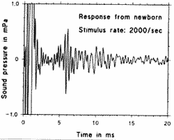
Figure 6a. Example of MLS derived OAE time-response from a newborn, measured with 60 dB p.e. SPL stimulus level, and recorded in linear mode.
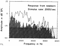
Figure 6b is the corresponding frequency spectrum showing a broad band response up to 4 kHz. The shaded arca represents the poise floor of the recording and the hatched part illustrates the sensitivity limit of the system.
The whole system is placed on a cart, and the preamplifier for the acoustic probe is mounted on a flexible arm for easy placement of the probe, and prohibiting the probe cable from touching clothes and other parts, which might disturb the measurements.
RESULTSThe system performance in an IEC-711 coupler can be seen from Figure 5, recorded in linear mode with a stimulus intensity of 60 dB SPL peak equivalent and 2000 stimulations/sec. The total number of stimulations is 122.600. The hatched area defines the limit of the sensitivity of the system (+/- 4 mPa), resulting from a combination of poise and distortion in the transducers. The frequency response for the total system is 700 - 6000 Hz (3 dB cut-off).
As an example a typical response from a newborn is shown in Figure 6a, recorded with a stimulus intensity of 60 dB SPL peak equivalent and a stimulus rate of 2000/ sec with a total of 1536 stimulations representing 6 sweeps of 256 clicks each. The actual measuring time in this example is thus less than one second. From the figure it can be seen, that the stimulus artifact has disappeared 3 to 4 ms after the stimulus onset. The corresponding frequency spectrum is depicted in Figure 6b, which shows a robust response up to 4 kHz, with some high frequency components around 6 kHz. The shaded area represents the poise floor and the hatched part illustrates thc sensitivity limit of the system.
The decrease in amplitude due to the increased stimulus rate was examined in a group of 17 normal hearing subjects (median age 31, range: 27-61, 10 males, 7 females). The rms mean value of the OAE-response in the time interval 5-20 ms after stimulus onset is shown in Figure 7. The error bars represent +/- 1 SD. From the figure it can be seen that the mean reduction of amplitude, when the stimulus rate is increased from 31 to 2004 clicks/s, is 66% with a range from 50 to 80% within +/- 1 SD.
In order to make a comparison between the conventional TEOAE and the response derived by MLS, TEOAE's were recorded on a conventional system (Madsen Electronics, Celesta 503) using the same probe in the same ear without refitting. A corresponding test with the same stimulus settings and a click rate of 31-.5 Hz was performed using the MLS system. The test group consisted of 11 normal hearing subjects (median age 42, range:8-61) with no history of hearing disorders. The median correlation coefficient from the test group was 0.75 (range 0.53 - 0.83).
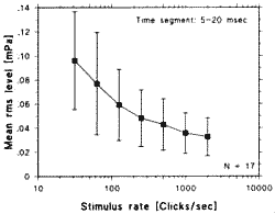
Figure 7. The rms mean- value of the OAE-response in the time interval 5-20 ms after stimulus onset. The error bars represent +/- 1 SD. The mean amplitude reduction, when the stimulus rate is increased from 31 to 2000 clicks/s, is 66% with a range from 50 to 80% within 1 SD.
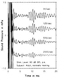
Figure 8. Linear recorded responses obtained in a normally hearing adult person at different stimulus rates. The morphology of the responses is mainly maintained in spite of the significant change in stimulus rate.
I he aim of this project was to provide a system for improved reliability of hearing screening in newborns using otoacoustic emissions. Applying the MLS technique has proved to be very efficient due to the highly reduced examination time, and the extended possibilities for noise cancellation and the optimisation of the signal to noise ratio.
Comparing measurements from conventional equipment and the MLS system showed good correlation between the two systems when the stimulus rate was within the same order of magnitude. The reason why the two responses were not identical, although recorded with the same probe in the same ear using identical stimulus parameters, is mainly due to differences in the filtering of the signals. Even if the cut-off frequencies are identical, the differences in phase shift will affect the shape of the time responses, unless the filters are of exactly the same type. The same phenomenon is also seen in brain stem response audiometry (Osterhammel 1981).
Using high stimulus rates will affect the amplitude of the responses as demonstrated by Thornton (1993). As seen from Figure 7 the amplitude reduction from conventional stimulus rates to the highest rate of 2000 clicks/s amounts to 66% on the average. This loss, however, is by lar compensated for by the improved speed of the test and the decreased noise level.
Figure 8 shown an example of recordings at different stimulus rates from a normal hearing adult subject. It seems like that the morphology of the responses is maintained in spite of the significant change in stimulus rate.
The introduction of the semi-non-linear method is an attempt to improve the distínction between the OAE response and the stimulus artifact. The criterion for the change between the non-linear and the linear part of the response was based on correlation calculations performed in selected time intervals. As mentioned earlier the coefficient chosen for the change-over was 0.6 based on experience achieved so far. Future analysis, based on a larger clinicai material, will prove whether this coefficíent is the optimal choice.
The MLS techníque is sensitive to the non-linearity of the transducers applied. As shown by Dunn (1993), nonlinear behaviour in MLS derived responses show up as artifacts sometimes very- late in the deconvoluted response (1012 ms after stimulus onset), with the risk of being mistaken as an OAE signal. Only by careful probe design and proper selection of the MLS sequences, this contribution of artifact signals can be reduced to below the practical noise limits.
CONCLUSIONA system for hearing screening of newborns using maximum length sequences as the stimulus signal has been described. The ability to obtain responses in noisy environments and in alert subjects is significantly improved by this system compared to conventional TEOAE equipment, due to the fast recording and the increased signal to noise ratio.
With the improved recording technique availabie, which also include the semi-non-linear recording technique, the possibility for reducing false positive and false negative results has been increased and the future efforts should therefore be focused on the interpretation of the emissions, which still is an essential problern due to the individual nature of otoacoustic emissions. The continuation of the present newborn screening project will concentrate on the analysis of the responses in order to improve the overall reliability of the screening test.
REFERENCESBRAY, P. - Click evoked otoacoustic emissions and the development of a clinical otoacoustic bearing test instrument. Doctoral thesis, University of London 1989.
DAVIES, W. D. T. - Generation and properties of maximumlength sequences - pari 1. Control., 10: 364-5, 1966. DUNN, C.; HAWKSFORD, M. O. - Distortion immunity of MLS-derived impulse response measurements. J. Audio Eng. Soc., 41: 314-35, 1993.
EYSHOLDT, U.; SCHREINER, C. - Maximum length sequences: A fast methoci for measuring brain-siem-evoked responses. Aadiology., 21: 242-50, 1982.
OSTERHAMMEL, P. A. - The unsolved problems in analog filtering on the auditory brain stem responses. Scand. Audiol., (Suppl. 13): 69-74, 1981.
THORNTON, A. R. D. - High rate otoacoustic emissions. J. Acoust. Soc. Am., 94: 132-6, 1993.
THORNTON, A. R. D.; FOLKARD, T. J.; CHAMBERS, J. D. - Technical aspects of recording evoked otoacoustic emissions using maximum length sequences. Scand. Audiol, 23: 22531, 1994.
Audiological Laboratory, Department of Otolaryngology Head and Neck Surgery - National University Hospital Rigshospitalet - Copenhagen, Denmark.
Address for off prints: Arne Norby Rasmussen - Audiological Laboratory, F 2072 - Dept. of otolaryngology, Head and Neck Surgery - Rigshospitalet, Blegdamsvej 9 - DK - 2100 Kbh. O. Artigo recebido em 26 de agosto de 1997. Artigo aceito em 15 de junho de 1998.